Steve Krawczyk, Director of Research & Development, Accelitas
At Accelitas, we’re dedicated to providing businesses with predictive insights that grow profitable accounts while reducing risks. And when it comes to the data analytics that deliver these insights, we believe in using the best tool for a job. To determine the best tool, you need to have well-rounded knowledge spanning multiple disciplines. It’s not sufficient simply to rely on one’s own area of expertise, even if that expertise includes PhD work. Work at the PhD level almost always requires specialization in a narrow topic within a single discipline. That tight focus is great for making incremental advances in a field of study. But it’s all too easy in post-graduate work to fall into the trap of keeping that tight focus when trying to solve the broad, highly varied range of problems that arise in the real world.
Artificial Intelligence (AI) has become a huge, internationally active field of study encompassing many approaches and applications. AI includes disciplines such as applied statistics, data mining, pattern recognition, machine learning, deep learning, probabilistic methods, and big data. Within these disciplines lie various sub-disciplines such as computer vision, image processing, natural language processing, and speech recognition. When applying AI to solve a problem, it is often beneficial to leverage techniques from more than one of these disciplines and sub-disciplines.
Applying a Cross-Disciplinary Approach
Here’s a simple example that demonstrates the benefits of taking a cross-disciplinary approach in AI. The figure below shows an artificial dataset containing two features (measured by the axes) and two classes (represented by the colored dots). Let’s say we want to analyze this data set to distinguish the purple class from the yellow class.
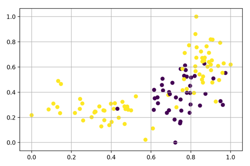
Figure 1: Sample data set
These types of distributions commonly appear when there are subpopulations within a feature.
In artificial intelligence, a feature is an individually measurable property or characteristic. For example, a person’s age could be a feature in an analysis of census data. In fact, age is a great example of data that might be represented in a plot like this, where people, say, less then 30 and greater than 60 perform similarly while those between 30 and 60 may differ. A similar distribution occurs for the feature on the x-axis in Figure 1 above. In this particular case, samples from 0-0.6 and 0.8-1.0 are similar while those with values 0.6-0.8 differ.
Obviously, these classes are not linearly separable; that is, you cannot draw a straight line neatly separating yellow from purple.
In AI terms, we would say that training a simple linear model on these two features completely fails. A simple linear model is a common starting place for modeling, whether one is modeling continuous data or categorical data, which is typically binary data or data with just two classes. In a linear model, each feature is assigned a single weight in the form of a coefficient. For example, if I have two features, x1 and x2, a linear model would take the form y = x1*c1 * x2*c2+b, where c1 and c2 are the learned coefficients (values suggested and then refined during analysis) and b is a constant (an offset along the y axis) that helps plotting the location of the line being modeled.
If we’re not going to use a linear model, how should we solve the problem? The answer to that question will depend on our expertise. And when it comes to expertise, the broader the better.
Some approaches to solving problems like the one shown in Figure 1 apply non-linear classifiers, such as neural networks or decision trees. There are also a number of alternatives, such as boosting (assigning weighted values to a feature to help with analysis), feature embedding, etc.
The main limitation with most of these approaches is that interpretability of the model is lost. In other words, once these approaches are applied, it’s no longer possible to determine why the classifier reached its decision.
Looking for Answers and Interpretability
Interpretability is one of the main advantages of linear classifiers. Their simplicity makes them easy to interpret. Having a model that is interpretable is extremely important (and often required) when using AI to make decisions that affect people, such as approving or denying loans.
I mentioned earlier the importance of having a broad, multi-disciplinary approach when it comes to AI. Here’s where that breadth really pays off.
It’s possible to use techniques from multiple AI disciplines to get accurate classification on the given dataset while still using a model that allows interpretability. One simple technique to allow non-linear separation of these features is to “bucket” them, transforming them into sparse features.
Bucketing? Sparse features? Let me explain.
Bucketing means slicing the feature according to its range. For example, if a feature varied from 0-100 and you used typical bucketing techniques to slice it up into 10 buckets, you would get 0-10, 11-20, ..., 91-100. Slicing data like this provides the most benefit for linear analysis if every bucket contains an equal number of samples.
A sparse feature is a feature with lots of missing values in its data set. For example, if you collected census data on 100 people and identified their occupations, and only 23 of them had the occupation of nurse, then the feature for the occupation of nurse would be a sparse feature. The feature is sparse, because it is positive (true) only a subset of the time.
Many big data techniques use very sparse features. (For example, a user’s web history is a sparse feature, since by necessity it contains a large number of null values representing sites never visited.) Sparse feature techniques are also applicable here. Why? Because we’re bucketing the data. Imagine a person whose age is 45. They would have a feature vector of [0,0,0,0,1,0,0,0,0,0]. The 1 would be for the 41-50 bucket while all other age buckets would be 0.
Rather than using simple bucketing techniques (with equally spaced buckets—that is, data subsets each having the same number of samples), performance can be greatly improved by analyzing the distribution of the feature to be bucketed. Leveraging applied statistics and, in particular, non-parametric modeling, the distribution of the features can be analyzed to find buckets that fit the data being analyzed.
Equally spaced buckets are suited for features that have a uniform distribution. This is usually not the case with real data, and it’s not the case for the sample data, as shown in the plots below.
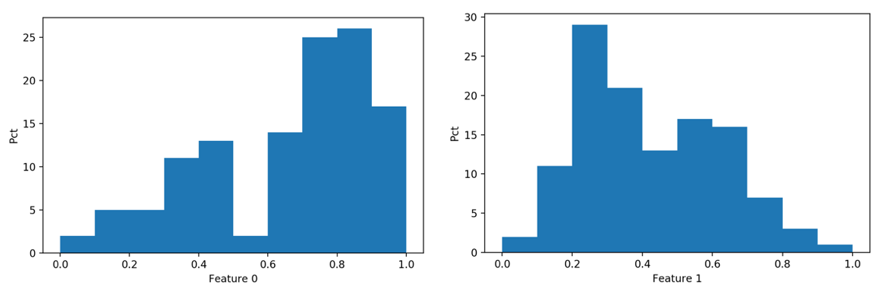
Figure 2: Bucketing data
The additional sparse features can be incorporated into the linear model, similar to kernel methods used in machine learning. (Kernel methods are algorithms for pattern analysis that can operate by applying a similarity function to two data points.) As mentioned, these solutions have now allowed a non-linear decision boundary in conjunction with a linear classifier. In other words, since a straight line could not accurately represent the distribution of our data, we are now able to accurately represent the distribution of the two classes with a non-linear decision boundary, which make take the form of a curved line or multiple lines. But we’re representing that non-linear boundary with a linear classifier so that our results will be interpretable.
The results are shown in the figure below. A decision boundary leveraging the feature extraction and modeling process described above is on the left (the linear classifier used was a logistic regression model). On the right is a decision boundary from a multilayer neural network (2 hidden layers with 10 and 4 neurons, respectively). The linear classifier obtains similar performance to the complex neural network, while supporting interpretability that the more complex neural network does not.
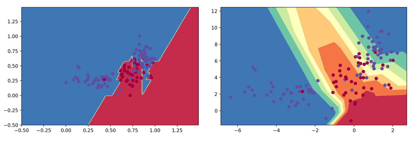
Figure 3: Representing that non-linear boundary with a linear classifier
Benefits of Leveraging from Multiple Disciplines in AI
This example showed the benefits of leveraging techniques from multiple disciplines within AI. Specifically:
- We leveraged techniques from big data to extract sparse features
- We leveraged applied statistics for modeling the distributions of the features in order to improve the extracted sparse features, and
- We combined these features with the original data to train a linear model, which is a common practice similar to kernel methods in machine learning.
Finally, we compared our process to the popular complex multi-layer neural networks, showing similar performance. Our results are predictive as those from neural networks, but unlike the results of neural networks, our results are interpretable.
From Many Techniques, an Interpretable and Predictive Answer
The end benefit of combining all these various techniques allowed the construction of a linear model that is able to learn complex decision boundaries. This is an important requirement for applications of AI where an explanation of the decision from the model is necessary. It allows easily interpretation for why an example was assigned a particular class.
At Accelitas, one of our primary focuses is to leverage AI to help lenders make more profitable decisions on loan applications and to streamline mobile account opening. Since lending decisions affect real people’s lives, it is critical we are able to explain why a decision was reached. Black box models (such as multi-layer neural networks) that return uninterpretable results are unusable for this use case. Accordingly, we lean on work done from various branches of AI to create models that are both powerful and interpretable.
The result in computer science terms is highly predictive analytics whose predictions can be explained. The result in real people’s lives is more loans granted to consumers and businesses, and higher profits and reduced losses for lenders. For everyone involved, it’s a highly beneficial use of AI.
Want to learn more about Accelitas predictive analytics?
Download our predictive analytics solution brief
by clicking the button below.